Regression Analysis in R Programming

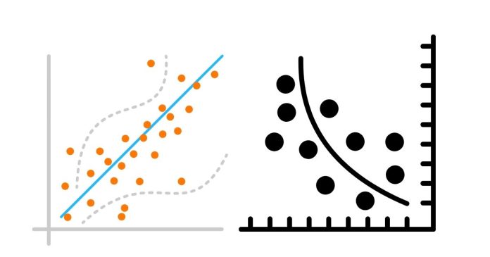
Regression analysis in R programming is a powerful way to examine relationships between variables. In R, you can perform regression analysis using several built-in functions and packages. Here’s a basic guide on how to do it:

1. Simple Linear Regression

Simple linear regression involves predicting one continuous dependent variable (Y) using one independent variable (X). The linear regression model assumes a relationship of the form: Y=β0+β1X+ϵY = \beta_0 + \beta_1 X + \epsilon

In R, you can use the lm() function to perform linear regression.

Example:

# Sample Data
x <- c(1, 2, 3, 4, 5)
y <- c(2, 4, 5, 4, 5)

# Fit the model
model <- lm(y ~ x)

# View summary of the model
summary(model)

• lm(y ~ x) fits a linear regression model with y as the dependent variable and x as the independent variable.
• summary(model) will show the coefficients, R-squared value, p-values, and other statistical details.

2. Multiple Linear Regression

Multiple linear regression is an extension where you predict the dependent variable using two or more independent variables.

Example:

# Sample Data
x1 <- c(1, 2, 3, 4, 5)
x2 <- c(5, 4, 3, 2, 1)
y <- c(2, 4, 5, 4, 5)

# Fit the model
model <- lm(y ~ x1 + x2)

# View summary of the model
summary(model)

3. Visualizing the Regression Line

You can visualize the regression model using plot() and abline() for simple linear regression.

Example:

# Simple linear regression plot
plot(x, y)
abline(model, col = "red")  # Add regression line

For multiple regression, you can use pairs plots or other visualizations like 3D plots for better interpretation.

4. Diagnostics and Model Checking

It’s essential to check for model assumptions like homoscedasticity, normality of residuals, and multicollinearity.

• Residual Plot: To check for constant variance.

plot(model$residuals)

• Q-Q Plot: To check if residuals follow a normal distribution.

qqnorm(model$residuals)
qqline(model$residuals)

• VIF (Variance Inflation Factor): To check for multicollinearity.

library(car)
vif(model)

5. R-Squared and Adjusted R-Squared

• R-squared: Measures the proportion of the variance in the dependent variable that is predictable from the independent variables.
• Adjusted R-squared: Adjusts the R-squared value based on the number of predictors to account for overfitting.

summary(model)$r.squared
summary(model)$adj.r.squared

6. Prediction with the Model

Once you have your model, you can make predictions for new data using the predict() function.

Example:

# New data for prediction
new_data <- data.frame(x1 = c(6, 7), x2 = c(0, -1))

# Predict using the model
predictions <- predict(model, newdata = new_data)

# View predictions
predictions

This should give you a solid foundation to perform regression analysis in R. Would you like more details or examples of a specific part of the process?