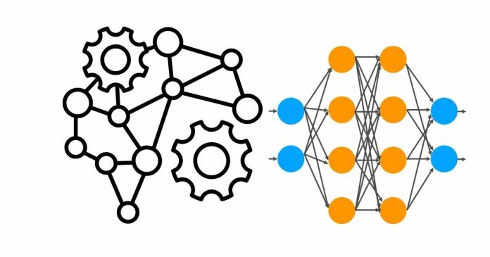
Backpropagation in Neural Network

Backpropagation is a fundamental algorithm used for training neural networks. It enables the network to learn from the errors it makes during training and adjust its parameters (weights and biases) to minimize the error in subsequent predictions. The process involves two main steps: forward propagation and backward propagation.

1. Forward Propagation:

In forward propagation, the input data is passed through the network layer by layer, applying weights and activation functions at each layer. The output is calculated based on the current weights and biases of the network.

2. Backward Propagation (Backpropagation):

Backpropagation is used to update the weights and biases in the network by minimizing the error between the predicted output and the actual output (ground truth). This process occurs in three main steps:

a. Calculate the Error:

First, the error is computed by comparing the network’s predicted output (from forward propagation) with the actual output. This is typically done using a loss function, such as Mean Squared Error (MSE) or Cross-Entropy Loss.

b. Compute Gradients:

Backpropagation uses the chain rule of calculus to compute the gradient (or partial derivatives) of the loss function with respect to each weight and bias in the network. This is done by propagating the error backward through the network, starting from the output layer and moving towards the input layer.

• Output Layer: The gradient of the loss with respect to the output is computed first.
• Hidden Layers: Gradients are then propagated backward through each hidden layer, adjusting each weight according to how much it contributed to the error.

c. Update Weights and Biases:

Once the gradients are computed, the weights and biases are updated using an optimization algorithm like Gradient Descent. The updates are proportional to the negative of the gradient, typically scaled by a learning rate, which controls the size of the update step.

Mathematically, the update rule for a weight ww is:

w=w−η⋅∂L∂ww = w – \eta \cdot \frac{\partial L}{\partial w}

Where:

• η\eta is the learning rate.
• ∂L∂w\frac{\partial L}{\partial w} is the gradient of the loss with respect to the weight ww.

Steps in Backpropagation:

1. Forward Pass: Compute the output of the network based on the input data.
2. Compute Loss: Calculate the difference between the predicted output and the actual target (loss).
3. Backward Pass: Compute the gradient of the loss with respect to each weight using the chain rule.
4. Update Weights: Use an optimization algorithm (e.g., Gradient Descent) to adjust the weights and biases.

Example in a Simple Neural Network:

Consider a neural network with one hidden layer:

• Input XX
• Hidden layer with activation function ff
• Output layer with activation gg

The steps are as follows:

• Forward Pass:
  • Calculate H=f(W1X+b1)H = f(W_1 X + b_1) (hidden layer output)
  • Calculate Y=g(W2H+b2)Y = g(W_2 H + b_2) (final output)
• Loss Calculation:
  • Use a loss function like MSE: L=12(Ypred−Ytrue)2L 
• Backpropagation:
  • Compute the gradient of the loss with respect to W2W_2, b2b_2, W1W_1, and b1b_1 using the chain rule.
• Weight Update:
  • Update W1W_1, W2W_2, b1b_1, and b2b_2 using the computed gradients and learning rate.

Importance of Backpropagation:

• It allows neural networks to learn complex patterns in data by iteratively adjusting the weights based on errors.
• The efficiency of backpropagation, especially when combined with optimization algorithms like Stochastic Gradient Descent (SGD), enables deep learning models to train on large datasets and perform well in tasks like image classification, speech recognition, and more.

Challenges:

• Vanishing and Exploding Gradients: In deep networks, gradients may become very small (vanish) or very large (explode), making training difficult.
• Local Minima: The network might get stuck in local minima, though techniques like stochastic gradient descent and modern optimizers help mitigate this.